Handwritten digit recognition is already widely used in the automatic processing of bank cheques, postal addresses, etc. Some of the existing systems include computational intelligence techniques such as artificial neural networks or fuzzy logic, whereas others may just be large lookup tables that contain possible realizations of handwritten digits.

Artificial neural networks have been developed since the 1940s, but only in the past fifteen years have they been widely applied in a large variety of disciplines. Originating from the artificial neuron, which is a simple mathematical model of a biological neuron, many varieties of neural networks exist nowadays. Although some are implemented in hardware, the majority are simulated in software.

Handwritten digit recognition is an important task in the field of computer vision and machine learning. It involves the ability of a machine to recognize handwritten digits, which can be useful in a wide range of applications such as postal automation, bank cheque processing, and signature recognition. Handwritten digit recognition has been a challenging problem for many years, but recent advancements in deep learning algorithms and computer hardware have made it possible to achieve high accuracy rates. In this blog post, we will explore the basics of handwritten digit recognition, the challenges involved, and the state-of-the-art techniques used to tackle this problem.

Handwritten digits classification using neural network

In this notebook, we will classify handwritten digits using a simple neural network that has only input and output layers. We will then add a hidden layer and see how the performance of the model improves. Handwritten digits classification using a neural network refers to the process of training a neural network to accurately classify handwritten digits. This is a common problem in the field of machine learning and computer vision and has applications in various areas such as postal automation, bank cheque processing, and signature recognition.

To perform handwritten digit classification using neural networks, the first step is to obtain a dataset of handwritten digit images. This dataset is typically divided into a training set and a testing set. The training set is used to train the neural network, while the testing set is used to evaluate its performance.

import tensorflow as tf
from tensorflow import keras
import matplotlib.pyplot as plt
%matplotlib inline
import numpy as np

(X_train, y_train) , (X_test, y_test) = keras.datasets.mnist.load_data()

len(X_train)

60000

len(X_test)

10000

X_train[0].shape

(28, 28)

X_train[0]

array([[ 0, 0, 0, 0, 0, 0, 0, 0, 0, 0, 0, 0, 0, 0, 0, 0, 0, 0, 0, 0, 0, 0, 0, 0, 0, 0, 0, 0], [ 0, 0, 0, 0, 0, 0, 0, 0, 0, 0, 0, 0, 0, 0, 0, 0, 0, 0, 0, 0, 0, 0, 0, 0, 0, 0, 0, 0], [ 0, 0, 0, 0, 0, 0, 0, 0, 0, 0, 0, 0, 0, 0, 0, 0, 0, 0, 0, 0, 0, 0, 0, 0, 0, 0, 0, 0], [ 0, 0, 0, 0, 0, 0, 0, 0, 0, 0, 0, 0, 0, 0, 0, 0, 0, 0, 0, 0, 0, 0, 0, 0, 0, 0, 0, 0], [ 0, 0, 0, 0, 0, 0, 0, 0, 0, 0, 0, 0, 0, 0, 0, 0, 0, 0, 0, 0, 0, 0, 0, 0, 0, 0, 0, 0], [ 0, 0, 0, 0, 0, 0, 0, 0, 0, 0, 0, 0, 3, 18, 18, 18, 126, 136, 175, 26, 166, 255, 247, 127, 0, 0, 0, 0], [ 0, 0, 0, 0, 0, 0, 0, 0, 30, 36, 94, 154, 170, 253, 253, 253, 253, 253, 225, 172, 253, 242, 195, 64, 0, 0, 0, 0], [ 0, 0, 0, 0, 0, 0, 0, 49, 238, 253, 253, 253, 253, 253, 253, 253, 253, 251, 93, 82, 82, 56, 39, 0, 0, 0, 0, 0], [ 0, 0, 0, 0, 0, 0, 0, 18, 219, 253, 253, 253, 253, 253, 198, 182, 247, 241, 0, 0, 0, 0, 0, 0, 0, 0, 0, 0], [ 0, 0, 0, 0, 0, 0, 0, 0, 80, 156, 107, 253, 253, 205, 11, 0, 43, 154, 0, 0, 0, 0, 0, 0, 0, 0, 0, 0], [ 0, 0, 0, 0, 0, 0, 0, 0, 0, 14, 1, 154, 253, 90, 0, 0, 0, 0, 0, 0, 0, 0, 0, 0, 0, 0, 0, 0], [ 0, 0, 0, 0, 0, 0, 0, 0, 0, 0, 0, 139, 253, 190, 2, 0, 0, 0, 0, 0, 0, 0, 0, 0, 0, 0, 0, 0], [ 0, 0, 0, 0, 0, 0, 0, 0, 0, 0, 0, 11, 190, 253, 70, 0, 0, 0, 0, 0, 0, 0, 0, 0, 0, 0, 0, 0], [ 0, 0, 0, 0, 0, 0, 0, 0, 0, 0, 0, 0, 35, 241, 225, 160, 108, 1, 0, 0, 0, 0, 0, 0, 0, 0, 0, 0], [ 0, 0, 0, 0, 0, 0, 0, 0, 0, 0, 0, 0, 0, 81, 240, 253, 253, 119, 25, 0, 0, 0, 0, 0, 0, 0, 0, 0], [ 0, 0, 0, 0, 0, 0, 0, 0, 0, 0, 0, 0, 0, 0, 45, 186, 253, 253, 150, 27, 0, 0, 0, 0, 0, 0, 0, 0], [ 0, 0, 0, 0, 0, 0, 0, 0, 0, 0, 0, 0, 0, 0, 0, 16, 93, 252, 253, 187, 0, 0, 0, 0, 0, 0, 0, 0], [ 0, 0, 0, 0, 0, 0, 0, 0, 0, 0, 0, 0, 0, 0, 0, 0, 0, 249, 253, 249, 64, 0, 0, 0, 0, 0, 0, 0], [ 0, 0, 0, 0, 0, 0, 0, 0, 0, 0, 0, 0, 0, 0, 46, 130, 183, 253, 253, 207, 2, 0, 0, 0, 0, 0, 0, 0], [ 0, 0, 0, 0, 0, 0, 0, 0, 0, 0, 0, 0, 39, 148, 229, 253, 253, 253, 250, 182, 0, 0, 0, 0, 0, 0, 0, 0], [ 0, 0, 0, 0, 0, 0, 0, 0, 0, 0, 24, 114, 221, 253, 253, 253, 253, 201, 78, 0, 0, 0, 0, 0, 0, 0, 0, 0], [ 0, 0, 0, 0, 0, 0, 0, 0, 23, 66, 213, 253, 253, 253, 253, 198, 81, 2, 0, 0, 0, 0, 0, 0, 0, 0, 0, 0], [ 0, 0, 0, 0, 0, 0, 18, 171, 219, 253, 253, 253, 253, 195, 80, 9, 0, 0, 0, 0, 0, 0, 0, 0, 0, 0, 0, 0], [ 0, 0, 0, 0, 55, 172, 226, 253, 253, 253, 253, 244, 133, 11, 0, 0, 0, 0, 0, 0, 0, 0, 0, 0, 0, 0, 0, 0], [ 0, 0, 0, 0, 136, 253, 253, 253, 212, 135, 132, 16, 0, 0, 0, 0, 0, 0, 0, 0, 0, 0, 0, 0, 0, 0, 0, 0], [ 0, 0, 0, 0, 0, 0, 0, 0, 0, 0, 0, 0, 0, 0, 0, 0, 0, 0, 0, 0, 0, 0, 0, 0, 0, 0, 0, 0], [ 0, 0, 0, 0, 0, 0, 0, 0, 0, 0, 0, 0, 0, 0, 0, 0, 0, 0, 0, 0, 0, 0, 0, 0, 0, 0, 0, 0], [ 0, 0, 0, 0, 0, 0, 0, 0, 0, 0, 0, 0, 0, 0, 0, 0, 0, 0, 0, 0, 0, 0, 0, 0, 0, 0, 0, 0]], dtype=uint8)

plt.matshow(X_train[0])

<matplotlib.image.AxesImage at 0x1fe79cb99e8>

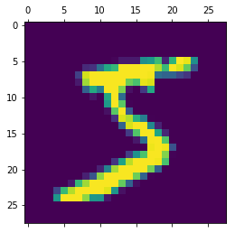
y_train[0]

5

X_train = X_train / 255
X_test = X_test / 255

X_train[0]

array([[0. , 0. , 0. , 0. , 0. , 0. , 0. , 0. , 0. , 0. , 0. , 0. , 0. , 0. , 0. , 0. , 0. , 0. , 0. , 0. , 0. , 0. , 0. , 0. , 0. , 0. , 0. , 0. ], [0. , 0. , 0. , 0. , 0. , 0. , 0. , 0. , 0. , 0. , 0. , 0. , 0. , 0. , 0. , 0. , 0. , 0. , 0. , 0. , 0. , 0. , 0. , 0. , 0. , 0. , 0. , 0. ], [0. , 0. , 0. , 0. , 0. , 0. , 0. , 0. , 0. , 0. , 0. , 0. , 0. , 0. , 0. , 0. , 0. , 0. , 0. , 0. , 0. , 0. , 0. , 0. , 0. , 0. , 0. , 0. ], [0. , 0. , 0. , 0. , 0. , 0. , 0. , 0. , 0. , 0. , 0. , 0. , 0. , 0. , 0. , 0. , 0. , 0. , 0. , 0. , 0. , 0. , 0. , 0. , 0. , 0. , 0. , 0. ], [0. , 0. , 0. , 0. , 0. , 0. , 0. , 0. , 0. , 0. , 0. , 0. , 0. , 0. , 0. , 0. , 0. , 0. , 0. , 0. , 0. , 0. , 0. , 0. , 0. , 0. , 0. , 0. ], [0. , 0. , 0. , 0. , 0. , 0. , 0. , 0. , 0. , 0. , 0. , 0. , 0.01176471, 0.07058824, 0.07058824, 0.07058824, 0.49411765, 0.53333333, 0.68627451, 0.10196078, 0.65098039, 1. , 0.96862745, 0.49803922, 0. , 0. , 0. , 0. ], [0. , 0. , 0. , 0. , 0. , 0. , 0. , 0. , 0.11764706, 0.14117647, 0.36862745, 0.60392157, 0.66666667, 0.99215686, 0.99215686, 0.99215686, 0.99215686, 0.99215686, 0.88235294, 0.6745098 , 0.99215686, 0.94901961, 0.76470588, 0.25098039, 0. , 0. , 0. , 0. ], [0. , 0. , 0. , 0. , 0. , 0. , 0. , 0.19215686, 0.93333333, 0.99215686, 0.99215686, 0.99215686, 0.99215686, 0.99215686, 0.99215686, 0.99215686, 0.99215686, 0.98431373, 0.36470588, 0.32156863, 0.32156863, 0.21960784, 0.15294118, 0. , 0. , 0. , 0. , 0. ], [0. , 0. , 0. , 0. , 0. , 0. , 0. , 0.07058824, 0.85882353, 0.99215686, 0.99215686, 0.99215686, 0.99215686, 0.99215686, 0.77647059, 0.71372549, 0.96862745, 0.94509804, 0. , 0. , 0. , 0. , 0. , 0. , 0. , 0. , 0. , 0. ], [0. , 0. , 0. , 0. , 0. , 0. , 0. , 0. , 0.31372549, 0.61176471, 0.41960784, 0.99215686, 0.99215686, 0.80392157, 0.04313725, 0. , 0.16862745, 0.60392157, 0. , 0. , 0. , 0. , 0. , 0. , 0. , 0. , 0. , 0. ], [0. , 0. , 0. , 0. , 0. , 0. , 0. , 0. , 0. , 0.05490196, 0.00392157, 0.60392157, 0.99215686, 0.35294118, 0. , 0. , 0. , 0. , 0. , 0. , 0. , 0. , 0. , 0. , 0. , 0. , 0. , 0. ], [0. , 0. , 0. , 0. , 0. , 0. , 0. , 0. , 0. , 0. , 0. , 0.54509804, 0.99215686, 0.74509804, 0.00784314, 0. , 0. , 0. , 0. , 0. , 0. , 0. , 0. , 0. , 0. , 0. , 0. , 0. ], [0. , 0. , 0. , 0. , 0. , 0. , 0. , 0. , 0. , 0. , 0. , 0.04313725, 0.74509804, 0.99215686, 0.2745098 , 0. , 0. , 0. , 0. , 0. , 0. , 0. , 0. , 0. , 0. , 0. , 0. , 0. ], [0. , 0. , 0. , 0. , 0. , 0. , 0. , 0. , 0. , 0. , 0. , 0. , 0.1372549 , 0.94509804, 0.88235294, 0.62745098, 0.42352941, 0.00392157, 0. , 0. , 0. , 0. , 0. , 0. , 0. , 0. , 0. , 0. ], [0. , 0. , 0. , 0. , 0. , 0. , 0. , 0. , 0. , 0. , 0. , 0. , 0. , 0.31764706, 0.94117647, 0.99215686, 0.99215686, 0.46666667, 0.09803922, 0. , 0. , 0. , 0. , 0. , 0. , 0. , 0. , 0. ], [0. , 0. , 0. , 0. , 0. , 0. , 0. , 0. , 0. , 0. , 0. , 0. , 0. , 0. , 0.17647059, 0.72941176, 0.99215686, 0.99215686, 0.58823529, 0.10588235, 0. , 0. , 0. , 0. , 0. , 0. , 0. , 0. ], [0. , 0. , 0. , 0. , 0. , 0. , 0. , 0. , 0. , 0. , 0. , 0. , 0. , 0. , 0. , 0.0627451 , 0.36470588, 0.98823529, 0.99215686, 0.73333333, 0. , 0. , 0. , 0. , 0. , 0. , 0. , 0. ], [0. , 0. , 0. , 0. , 0. , 0. , 0. , 0. , 0. , 0. , 0. , 0. , 0. , 0. , 0. , 0. , 0. , 0.97647059, 0.99215686, 0.97647059, 0.25098039, 0. , 0. , 0. , 0. , 0. , 0. , 0. ], [0. , 0. , 0. , 0. , 0. , 0. , 0. , 0. , 0. , 0. , 0. , 0. , 0. , 0. , 0.18039216, 0.50980392, 0.71764706, 0.99215686, 0.99215686, 0.81176471, 0.00784314, 0. , 0. , 0. , 0. , 0. , 0. , 0. ], [0. , 0. , 0. , 0. , 0. , 0. , 0. , 0. , 0. , 0. , 0. , 0. , 0.15294118, 0.58039216, 0.89803922, 0.99215686, 0.99215686, 0.99215686, 0.98039216, 0.71372549, 0. , 0. , 0. , 0. , 0. , 0. , 0. , 0. ], [0. , 0. , 0. , 0. , 0. , 0. , 0. , 0. , 0. , 0. , 0.09411765, 0.44705882, 0.86666667, 0.99215686, 0.99215686, 0.99215686, 0.99215686, 0.78823529, 0.30588235, 0. , 0. , 0. , 0. , 0. , 0. , 0. , 0. , 0. ], [0. , 0. , 0. , 0. , 0. , 0. , 0. , 0. , 0.09019608, 0.25882353, 0.83529412, 0.99215686, 0.99215686, 0.99215686, 0.99215686, 0.77647059, 0.31764706, 0.00784314, 0. , 0. , 0. , 0. , 0. , 0. , 0. , 0. , 0. , 0. ], [0. , 0. , 0. , 0. , 0. , 0. , 0.07058824, 0.67058824, 0.85882353, 0.99215686, 0.99215686, 0.99215686, 0.99215686, 0.76470588, 0.31372549, 0.03529412, 0. , 0. , 0. , 0. , 0. , 0. , 0. , 0. , 0. , 0. , 0. , 0. ], [0. , 0. , 0. , 0. , 0.21568627, 0.6745098 , 0.88627451, 0.99215686, 0.99215686, 0.99215686, 0.99215686, 0.95686275, 0.52156863, 0.04313725, 0. , 0. , 0. , 0. , 0. , 0. , 0. , 0. , 0. , 0. , 0. , 0. , 0. , 0. ], [0. , 0. , 0. , 0. , 0.53333333, 0.99215686, 0.99215686, 0.99215686, 0.83137255, 0.52941176, 0.51764706, 0.0627451 , 0. , 0. , 0. , 0. , 0. , 0. , 0. , 0. , 0. , 0. , 0. , 0. , 0. , 0. , 0. , 0. ], [0. , 0. , 0. , 0. , 0. , 0. , 0. , 0. , 0. , 0. , 0. , 0. , 0. , 0. , 0. , 0. , 0. , 0. , 0. , 0. , 0. , 0. , 0. , 0. , 0. , 0. , 0. , 0. ], [0. , 0. , 0. , 0. , 0. , 0. , 0. , 0. , 0. , 0. , 0. , 0. , 0. , 0. , 0. , 0. , 0. , 0. , 0. , 0. , 0. , 0. , 0. , 0. , 0. , 0. , 0. , 0. ], [0. , 0. , 0. , 0. , 0. , 0. , 0. , 0. , 0. , 0. , 0. , 0. , 0. , 0. , 0. , 0. , 0. , 0. , 0. , 0. , 0. , 0. , 0. , 0. , 0. , 0. , 0. , 0. ]])

X_train_flattened = X_train.reshape(len(X_train), 28*28)
X_test_flattened = X_test.reshape(len(X_test), 28*28)

X_train_flattened.shape

(60000, 784)

X_train_flattened[0]

array([0. , 0. , 0. , 0. , 0. , 0. , 0. , 0. , 0. , 0. , 0. , 0. , 0. , 0. , 0. , 0. , 0. , 0. , 0. , 0. , 0. , 0. , 0. , 0. , 0. , 0. , 0. , 0. , 0. , 0. , 0. , 0. , 0. , 0. , 0. , 0. , 0. , 0. , 0. , 0. , 0. , 0. , 0. , 0. , 0. , 0. , 0. , 0. , 0. , 0. , 0. , 0. , 0. , 0. , 0. , 0. , 0. , 0. , 0. , 0. , 0. , 0. , 0. , 0. , 0. , 0. , 0. , 0. , 0. , 0. , 0. , 0. , 0. , 0. , 0. , 0. , 0. , 0. , 0. , 0. , 0. , 0. , 0. , 0. , 0. , 0. , 0. , 0. , 0. , 0. , 0. , 0. , 0. , 0. , 0. , 0. , 0. , 0. , 0. , 0. , 0. , 0. , 0. , 0. , 0. , 0. , 0. , 0. , 0. , 0. , 0. , 0. , 0. , 0. , 0. , 0. , 0. , 0. , 0. , 0. , 0. , 0. , 0. , 0. , 0. , 0. , 0. , 0. , 0. , 0. , 0. , 0. , 0. , 0. , 0. , 0. , 0. , 0. , 0. , 0. , 0. , 0. , 0. , 0. , 0. , 0. , 0. , 0. , 0. , 0. , 0. , 0. , 0.01176471, 0.07058824, 0.07058824, 0.07058824, 0.49411765, 0.53333333, 0.68627451, 0.10196078, 0.65098039, 1. , 0.96862745, 0.49803922, 0. , 0. , 0. , 0. , 0. , 0. , 0. , 0. , 0. , 0. , 0. , 0. , 0.11764706, 0.14117647, 0.36862745, 0.60392157, 0.66666667, 0.99215686, 0.99215686, 0.99215686, 0.99215686, 0.99215686, 0.88235294, 0.6745098 , 0.99215686, 0.94901961, 0.76470588, 0.25098039, 0. , 0. , 0. , 0. , 0. , 0. , 0. , 0. , 0. , 0. , 0. , 0.19215686, 0.93333333, 0.99215686, 0.99215686, 0.99215686, 0.99215686, 0.99215686, 0.99215686, 0.99215686, 0.99215686, 0.98431373, 0.36470588, 0.32156863, 0.32156863, 0.21960784, 0.15294118, 0. , 0. , 0. , 0. , 0. , 0. , 0. , 0. , 0. , 0. , 0. , 0. , 0.07058824, 0.85882353, 0.99215686, 0.99215686, 0.99215686, 0.99215686, 0.99215686, 0.77647059, 0.71372549, 0.96862745, 0.94509804, 0. , 0. , 0. , 0. , 0. , 0. , 0. , 0. , 0. , 0. , 0. , 0. , 0. , 0. , 0. , 0. , 0. , 0. , 0.31372549, 0.61176471, 0.41960784, 0.99215686, 0.99215686, 0.80392157, 0.04313725, 0. , 0.16862745, 0.60392157, 0. , 0. , 0. , 0. , 0. , 0. , 0. , 0. , 0. , 0. , 0. , 0. , 0. , 0. , 0. , 0. , 0. , 0. , 0. , 0.05490196, 0.00392157, 0.60392157, 0.99215686, 0.35294118, 0. , 0. , 0. , 0. , 0. , 0. , 0. , 0. , 0. , 0. , 0. , 0. , 0. , 0. , 0. , 0. , 0. , 0. , 0. , 0. , 0. , 0. , 0. , 0. , 0. , 0.54509804, 0.99215686, 0.74509804, 0.00784314, 0. , 0. , 0. , 0. , 0. , 0. , 0. , 0. , 0. , 0. , 0. , 0. , 0. , 0. , 0. , 0. , 0. , 0. , 0. , 0. , 0. , 0. , 0. , 0. , 0.04313725, 0.74509804, 0.99215686, 0.2745098 , 0. , 0. , 0. , 0. , 0. , 0. , 0. , 0. , 0. , 0. , 0. , 0. , 0. , 0. , 0. , 0. , 0. , 0. , 0. , 0. , 0. , 0. , 0. , 0. , 0. , 0.1372549 , 0.94509804, 0.88235294, 0.62745098, 0.42352941, 0.00392157, 0. , 0. , 0. , 0. , 0. , 0. , 0. , 0. , 0. , 0. , 0. , 0. , 0. , 0. , 0. , 0. , 0. , 0. , 0. , 0. , 0. , 0. , 0. , 0.31764706, 0.94117647, 0.99215686, 0.99215686, 0.46666667, 0.09803922, 0. , 0. , 0. , 0. , 0. , 0. , 0. , 0. , 0. , 0. , 0. , 0. , 0. , 0. , 0. , 0. , 0. , 0. , 0. , 0. , 0. , 0. , 0. , 0.17647059, 0.72941176, 0.99215686, 0.99215686, 0.58823529, 0.10588235, 0. , 0. , 0. , 0. , 0. , 0. , 0. , 0. , 0. , 0. , 0. , 0. , 0. , 0. , 0. , 0. , 0. , 0. , 0. , 0. , 0. , 0. , 0. , 0.0627451 , 0.36470588, 0.98823529, 0.99215686, 0.73333333, 0. , 0. , 0. , 0. , 0. , 0. , 0. , 0. , 0. , 0. , 0. , 0. , 0. , 0. , 0. , 0. , 0. , 0. , 0. , 0. , 0. , 0. , 0. , 0. , 0. , 0.97647059, 0.99215686, 0.97647059, 0.25098039, 0. , 0. , 0. , 0. , 0. , 0. , 0. , 0. , 0. , 0. , 0. , 0. , 0. , 0. , 0. , 0. , 0. , 0. , 0. , 0. , 0. , 0.18039216, 0.50980392, 0.71764706, 0.99215686, 0.99215686, 0.81176471, 0.00784314, 0. , 0. , 0. , 0. , 0. , 0. , 0. , 0. , 0. , 0. , 0. , 0. , 0. , 0. , 0. , 0. , 0. , 0. , 0. , 0.15294118, 0.58039216, 0.89803922, 0.99215686, 0.99215686, 0.99215686, 0.98039216, 0.71372549, 0. , 0. , 0. , 0. , 0. , 0. , 0. , 0. , 0. , 0. , 0. , 0. , 0. , 0. , 0. , 0. , 0. , 0. , 0.09411765, 0.44705882, 0.86666667, 0.99215686, 0.99215686, 0.99215686, 0.99215686, 0.78823529, 0.30588235, 0. , 0. , 0. , 0. , 0. , 0. , 0. , 0. , 0. , 0. , 0. , 0. , 0. , 0. , 0. , 0. , 0. , 0.09019608, 0.25882353, 0.83529412, 0.99215686, 0.99215686, 0.99215686, 0.99215686, 0.77647059, 0.31764706, 0.00784314, 0. , 0. , 0. , 0. , 0. , 0. , 0. , 0. , 0. , 0. , 0. , 0. , 0. , 0. , 0. , 0. , 0.07058824, 0.67058824, 0.85882353, 0.99215686, 0.99215686, 0.99215686, 0.99215686, 0.76470588, 0.31372549, 0.03529412, 0. , 0. , 0. , 0. , 0. , 0. , 0. , 0. , 0. , 0. , 0. , 0. , 0. , 0. , 0. , 0. , 0.21568627, 0.6745098 , 0.88627451, 0.99215686, 0.99215686, 0.99215686, 0.99215686, 0.95686275, 0.52156863, 0.04313725, 0. , 0. , 0. , 0. , 0. , 0. , 0. , 0. , 0. , 0. , 0. , 0. , 0. , 0. , 0. , 0. , 0. , 0. , 0.53333333, 0.99215686, 0.99215686, 0.99215686, 0.83137255, 0.52941176, 0.51764706, 0.0627451 , 0. , 0. , 0. , 0. , 0. , 0. , 0. , 0. , 0. , 0. , 0. , 0. , 0. , 0. , 0. , 0. , 0. , 0. , 0. , 0. , 0. , 0. , 0. , 0. , 0. , 0. , 0. , 0. , 0. , 0. , 0. , 0. , 0. , 0. , 0. , 0. , 0. , 0. , 0. , 0. , 0. , 0. , 0. , 0. , 0. , 0. , 0. , 0. , 0. , 0. , 0. , 0. , 0. , 0. , 0. , 0. , 0. , 0. , 0. , 0. , 0. , 0. , 0. , 0. , 0. , 0. , 0. , 0. , 0. , 0. , 0. , 0. , 0. , 0. , 0. , 0. , 0. , 0. , 0. , 0. , 0. , 0. , 0. , 0. , 0. , 0. , 0. , 0. , 0. , 0. , 0. , 0. , 0. , 0. , 0. , 0. , 0. , 0. , 0. , 0. ])

Overall, handwritten digits classification using neural networks is a powerful and widely used technique in the field of machine learning and computer vision. It has numerous practical applications, and continues to be an active area of research and development.

Very simple neural network with no hidden layers

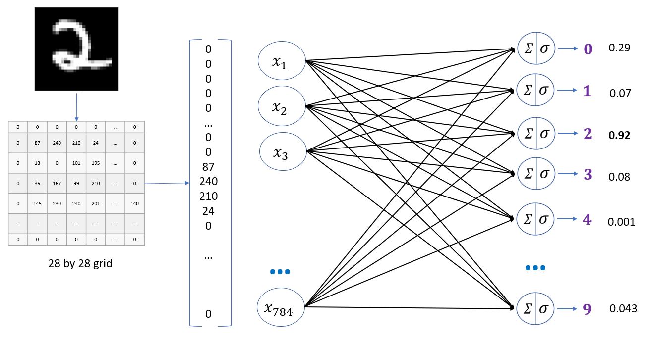
A very simple neural network with no hidden layers, also known as a single-layer perceptron, is a basic type of neural network architecture that consists of only one layer of neurons. This type of neural network is commonly used for binary classification problems, where the goal is to classify input data into one of two categories.

In a single-layer perceptron, the input data is fed into the input layer, which is directly connected to the output layer. The output layer computes a weighted sum of the input features, applies an activation function to the sum, and produces a single output value. This output value is then used to classify the input into one of the two categories.

Unlike more complex neural networks that have hidden layers, a single-layer perceptron does not have the ability to learn complex representations of the input data. Instead, it is limited to linear decision boundaries between the two classes. This makes it a simple and computationally efficient neural network architecture that can be trained quickly and easily.

Single-layer perceptrons have been used in a variety of applications, such as image and speech recognition, and they have also been used as a building block for more complex neural network architectures. However, due to their simplicity and limited capabilities, they are not well-suited for tasks that require more complex decision boundaries and non-linear relationships between the input features and the output.

model = keras.Sequential([
    keras.layers.Dense(10, input_shape=(784,), activation='sigmoid')
])

model.compile(optimizer='adam',
              loss='sparse_categorical_crossentropy',
              metrics=['accuracy'])

model.fit(X_train_flattened, y_train, epochs=5)

Epoch 1/5 1875/1875 [==============================] - 3s 1ms/step - loss: 0.4886 - accuracy: 0.8775 Epoch 2/5 1875/1875 [==============================] - 3s 1ms/step - loss: 0.3060 - accuracy: 0.9156 Epoch 3/5 1875/1875 [==============================] - 2s 1ms/step - loss: 0.2848 - accuracy: 0.9214 Epoch 4/5 1875/1875 [==============================] - 2s 1ms/step - loss: 0.2747 - accuracy: 0.9243 Epoch 5/5 1875/1875 [==============================] - 2s 1ms/step - loss: 0.2677 - accuracy: 0.9262

<tensorflow.python.keras.callbacks.History at 0x1fe24f47a90>

model.evaluate(X_test_flattened, y_test)

313/313 [==============================] - 0s 985us/step - loss: 0.2670 - Accuracy: 0.9257

[0.26697656512260437, 0.9257000088691711]

y_predicted = model.predict(X_test_flattened)
y_predicted[0]

array([1.7270680e-05, 1.3593615e-10, 4.5622761e-05, 7.5602829e-03, 1.3076769e-06, 7.5061922e-05, 1.7646971e-09, 6.9968843e-01, 7.8440302e-05, 8.1232190e-04], dtype=float32)

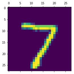
plt.matshow(X_test[0])

<matplotlib.image.AxesImage at 0x1fe2322e3c8>

np.argmax finds a maximum element from an array and returns the index of it

np.argmax(y_predicted[0])

7

y_predicted_labels = [np.argmax(i) for i in y_predicted]

y_predicted_labels[:5]

[7, 2, 1, 0, 4]

cm = tf.math.confusion_matrix(labels=y_test,predictions=y_predicted_labels)
cm

<tf.Tensor: shape=(10, 10), dtype=int32, numpy= array([[ 960, 0, 0, 2, 0, 5, 10, 2, 1, 0], [ 0, 1109, 3, 2, 0, 1, 4, 2, 14, 0], [ 7, 7, 929, 11, 5, 4, 15, 8, 42, 4], [ 3, 0, 23, 910, 0, 27, 6, 11, 23, 7], [ 1, 1, 2, 1, 915, 0, 16, 4, 10, 32], [ 11, 2, 2, 27, 9, 773, 23, 4, 33, 8], [ 7, 3, 5, 1, 7, 7, 925, 2, 1, 0], [ 1, 6, 25, 5, 8, 0, 0, 941, 2, 40], [ 7, 5, 7, 18, 9, 22, 11, 8, 880, 7], [ 11, 7, 1, 10, 32, 6, 0, 18, 9, 915]])>

import seaborn as sn
plt.figure(figsize = (10,7))
sn.heatmap(cm, annot=True, fmt='d')
plt.xlabel('Predicted')
plt.ylabel('Truth')

Text(69.0, 0.5, 'Truth')

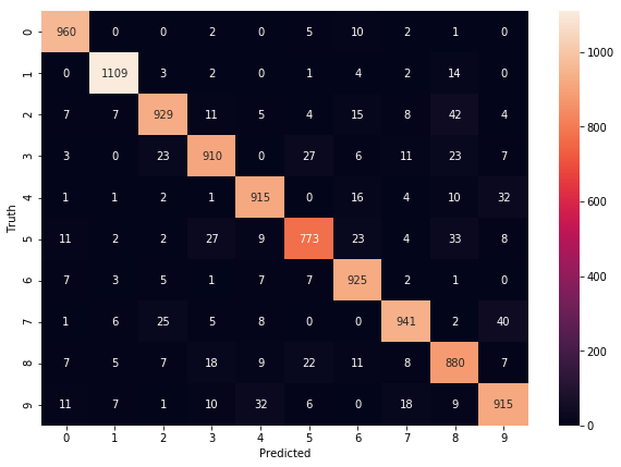
Overall, a very simple neural network with no hidden layers is a basic type of neural network architecture that can be used for simple binary classification tasks. While it has limitations in terms of its ability to learn complex representations, it is a useful and accessible tool for researchers and developers who are interested in exploring the fundamentals of neural networks.

Using hidden layer

Using hidden layers refers to the technique of incorporating one or more hidden layers in a neural network architecture. Hidden layers are layers of neurons that are not directly connected to the input or output layers of the neural network, and their purpose is to learn more complex representations of the input data.

In a neural network with hidden layers, the input data is fed into the input layer, and then passed through one or more hidden layers before reaching the output layer. Each hidden layer performs a series of nonlinear transformations on the input data, allowing the neural network to learn more complex representations of the input features.

The number of hidden layers and the number of neurons in each layer are hyperparameters that need to be chosen carefully to ensure that the neural network can learn useful representations of the input data without overfitting to the training data. This process of choosing the optimal hyperparameters is often done through a process of trial and error or through the use of automated techniques such as grid search or random search.

The use of hidden layers has been shown to be highly effective in a wide range of applications, including image recognition, natural language processing, and speech recognition. By allowing neural networks to learn more complex representations of the input data, hidden layers enable neural networks to achieve higher levels of accuracy and robustness than would be possible with a simple network architecture.

model = keras.Sequential([
    keras.layers.Dense(100, input_shape=(784,), activation='relu'),
    keras.layers.Dense(10, activation='sigmoid')
])

model.compile(optimizer='adam',
              loss='sparse_categorical_crossentropy',
              metrics=['accuracy'])

model.fit(X_train_flattened, y_train, epochs=5)

Epoch 1/5 1875/1875 [==============================] - 3s 2ms/step - loss: 0.2925 - accuracy: 0.9191 Epoch 2/5 1875/1875 [==============================] - 3s 2ms/step - loss: 0.1366 - accuracy: 0.9602 Epoch 3/5 1875/1875 [==============================] - 3s 2ms/step - loss: 0.0981 - accuracy: 0.9703 Epoch 4/5 1875/1875 [==============================] - 3s 2ms/step - loss: 0.0764 - accuracy: 0.9768 Epoch 5/5 1875/1875 [==============================] - 3s 2ms/step - loss: 0.0618 - accuracy: 0.9812

<tensorflow.python.keras.callbacks.History at 0x1fe230e7128>

model.evaluate(X_test_flattened,y_test)

313/313 [==============================] - 0s 1ms/step - loss: 0.0966 - Accuracy: 0.9716

[0.09658893942832947, 0.9715999960899353]

y_predicted = model.predict(X_test_flattened)
y_predicted_labels = [np.argmax(i) for i in y_predicted]
cm = tf.math.confusion_matrix(labels=y_test,predictions=y_predicted_labels)

plt.figure(figsize = (10,7))
sn.heatmap(cm, annot=True, fmt='d')
plt.xlabel('Predicted')
plt.ylabel('Truth')

Text(69.0, 0.5, 'Truth')

Overall, using hidden layers is an essential technique for building powerful neural network architectures that can learn complex relationships between input features and output targets. With the help of hidden layers, neural networks can learn to recognize patterns in data that would be difficult or impossible to detect using simpler techniques.

Using Flatten layer so that we don't have to call .reshape on the input dataset

Using a Flatten layer in a neural network architecture is a technique that allows us to simplify the input data by flattening it into a one-dimensional vector, without having to manually reshape the input dataset. This can be particularly useful when working with high-dimensional data, such as images, where it can be difficult to keep track of the shape of the input dataset as it moves through the network.

The Flatten layer is typically used after the convolutional layers in a convolutional neural network (CNN) architecture. The convolutional layers extract features from the input image, and the Flatten layer then flattens the output of the convolutional layers into a one-dimensional vector, which can be fed into a fully connected layer for classification or regression.

By using a Flatten layer, we can simplify the input data and reduce the complexity of the network architecture. This can lead to faster training times and better performance, especially when working with large datasets. Additionally, by automating the process of flattening the input data, we can reduce the risk of errors and make the code more efficient and easier to read.

model = keras.Sequential([
    keras.layers.Flatten(input_shape=(28, 28)),
    keras.layers.Dense(100, activation='relu'),
    keras.layers.Dense(10, activation='sigmoid')
])

model.compile(optimizer='adam',
              loss='sparse_categorical_crossentropy',
              metrics=['accuracy'])

model.fit(X_train, y_train, epochs=10)

Epoch 1/10 1875/1875 [==============================] - 3s 2ms/step - loss: 0.2959 - accuracy: 0.9185 Epoch 2/10 1875/1875 [==============================] - 3s 2ms/step - loss: 0.1368 - accuracy: 0.9603 Epoch 3/10 1875/1875 [==============================] - 3s 2ms/step - loss: 0.0995 - accuracy: 0.9703 Epoch 4/10 1875/1875 [==============================] - 3s 2ms/step - loss: 0.0771 - accuracy: 0.9772 Epoch 5/10 1875/1875 [==============================] - 3s 2ms/step - loss: 0.0628 - accuracy: 0.9806 Epoch 6/10 1875/1875 [==============================] - 3s 2ms/step - loss: 0.0519 - accuracy: 0.9841 Epoch 7/10 1875/1875 [==============================] - 3s 2ms/step - loss: 0.0442 - accuracy: 0.9865 Epoch 8/10 1875/1875 [==============================] - 3s 2ms/step - loss: 0.0369 - accuracy: 0.9886 Epoch 9/10 1875/1875 [==============================] - 3s 2ms/step - loss: 0.0300 - accuracy: 0.9910 Epoch 10/10 1875/1875 [==============================] - 3s 2ms/step - loss: 0.0264 - accuracy: 0.9917

<tensorflow.python.keras.callbacks.History at 0x1fe24629e80>

model.evaluate(X_test,y_test)

313/313 [==============================] - 0s 1ms/step - loss: 0.0813 - Accuracy: 0.9779

[0.08133944123983383, 0.9779000282287598]

Overall, using a Flatten layer in a neural network architecture is a useful technique for simplifying the input data and improving the performance of the network. By eliminating the need to manually reshape the input dataset, we can streamline the process of building and training neural networks, making it easier and more efficient to work with high-dimensional data.

Overall Conclusion

In conclusion, handwritten digit recognition is an important problem in the field of computer vision and machine learning. With recent advancements in deep learning algorithms and computer hardware, it is now possible to achieve high accuracy rates on this task. Handwritten digit recognition has a wide range of applications, from postal automation to signature recognition, and will continue to be an important area of research and development in the future. We hope this blog post has provided you with a basic understanding of the problem and the techniques used to solve it.

"THANK YOU!"