

Data Visualisation: An attractive way to present data!

Hey there!👋 I'm Vedant Pandya (He/Him) – a passionate explorer at the intersection of technology and innovation. With a robust background in Machine Learning, Generative Artificial Intelligence (Gen AI), Data Science, and Cloud Computing (both AWS and GCP), I've immersed myself in the dynamic realm of Industry 4.0 for over 4 years.
As a trailblazing Machine Learning Engineer and Data Scientist, I thrive on translating complex concepts into tangible solutions. My journey spans diverse sectors, from consulting to industry to tech, and I've championed cutting-edge open-source projects from inception to reality.
An advocate of continuous learning and growth, I'm deeply committed to fostering development and mentoring. I spearhead impactful learning initiatives within workplaces and academic institutions, empowering individuals to exceed their perceived limits.
Certified by Google Cloud in Machine Learning and Data Science (MOOC - @Coursera), I'm also honored to be a Google Women TechMaker. I channel my insights as a content creator and blogger, shedding light on intricate tech nuances.
My academic prowess shines with a Bachelor's degree in Information Technology, marked by distinction. Beyond the professional realm, I carry the pride of being raised by a single parent, instilled with values of dignity and resilience.
Expertise: 🚀 Industry 4.0 Visionary 🔍 NLP & Computer Vision Aficionado / Virtuoso ☁️ Google Cloud Advocate 🛠️ AI & ML Architect 🌱 Empowering Mentor 🌟 Deep Learning Maven 🎮 Reinforcement Learning Connoisseur 🌌 Quantum Computing Trailblazer 🌐 Edge Computing Advocate
Feel free to connect for invigorating conversations on AI, Machine Learning, Data Science, Quantum Computing, or the expansive world of Cloud Computing. Let's embark on a journey to unveil your latent potential 🚀
Remember, all perspectives shared are exclusively mine and do not mirror the viewpoints of my employer.Key Words: AI Innovation, Cloud Pioneering, Tech Mentorship, Cutting-Edge ML, Strategic Partnerships, Quantum Leap in Tech, AI Advancements, Cloud Empowerment, Mentorship in Innovation, Industry 4.0, Natural Language Processing, Computer Vision, AWS & Google Cloud, Machine Learning, Artificial Intelligence (AI/ML), Program Management, Data Science, Google Cloud, AWS, Solutions Architecture, Personal Development, AI, ML & Automation, Strategic Partnership, Strategy Consulting.
Hello, Folks!
I am a Student who's practicing Data Science, Machine Learning, Deep Learning and Artificial Intelligence with Cloud Computing Platform.
In this article, we are going to discuss the Data Visualisation techniques and how to implement them with simple steps. I am going to demonstrate the basic Data Visualisation techniques.
What is Data Visualisation?
There are two definitions for that:
First, in simple words, it is a technique to represent the data in picturized form.
Second, in technical words, it is the Graphical Representation of information and data. By using visual elements like charts, graphs, and maps, data visualization tools provide an accessible way to see and understand trends, outliers, and patterns in data.
There are many libraries that are used in data visualization. If you are a beginner then start with the seaborn and matplotlib. I am going to use these two here.
SO, let's go through the requirements first
Download and install it with the commands provided
Libraries Used:
For Data Visualisation:
- SeaBorn
pip install seaborn
- MatPlotLib
pip install matplotlib
For Data Analysis and Manipulation:
pip install pandas
Dataset:
Click on the dataset and download it. Keep it in the same folder which contains your .ipynb file.
Let's Start!
Import the required libraries and data set.
Then with the object_name.head() function, we can print the first five lines of the dataset to check whether it's imported properly or not.
import pandas as pd
import warnings
warnings.filterwarnings("ignore")
import seaborn as sns
import matplotlib.pyplot as plt
sns.set(style="white", color_codes=True)
iris = pd.read_csv("iris.csv")
iris.head()
| Id | SepalLengthCm | SepalWidthCm | PetalLengthCm | PetalWidthCm | Species | |
|---|---|---|---|---|---|---|
| 0 | 1 | 5.1 | 3.5 | 1.4 | 0.2 | Iris-setosa |
| 1 | 2 | 4.9 | 3.0 | 1.4 | 0.2 | Iris-setosa |
| 2 | 3 | 4.7 | 3.2 | 1.3 | 0.2 | Iris-setosa |
| 3 | 4 | 4.6 | 3.1 | 1.5 | 0.2 | Iris-setosa |
| 4 | 5 | 5.0 | 3.6 | 1.4 | 0.2 | Iris-setosa |
Now, check the total number of values that are present there in the given dataset with the object_name.count() function.
iris["Species"].value_counts()
Output:
Iris-virginica     50
Iris-versicolor    50
Iris-setosa        50
Name: Species, dtype: int64
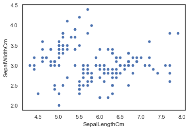
Now, let's plot the Scatter Plot with SepalLength on X_Axis and SepalWidth on Y_Axis.
iris.plot(kind="scatter", x="SepalLengthCm", y="SepalWidthCm")
Output:
*c* argument looks like a single numeric RGB or RGBA sequence, which should be avoided as value-mapping will have precedence in case its length matches with *x* & *y*.  Please use the *color* keyword-argument or provide a 2-D array with a single row if you intend to specify the same RGB or RGBA value for all points.


<AxesSubplot:xlabel='SepalLengthCm', ylabel='SepalWidthCm'>
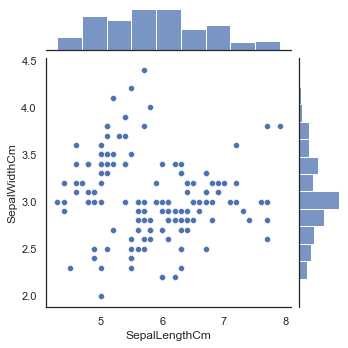
sns.jointplot(x="SepalLengthCm", y="SepalWidthCm", data=iris, size=5)
Output:
<seaborn.axisgrid.JointGrid at 0x11a2a170>
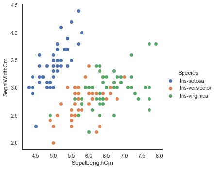
sns.FacetGrid(iris, hue="Species", size=5) \
   .map(plt.scatter, "SepalLengthCm", "SepalWidthCm") \
   .add_legend()
Output:
<seaborn.axisgrid.FacetGrid at 0x11b8ced0>
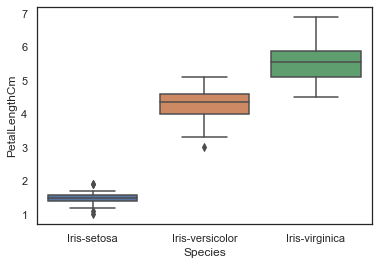
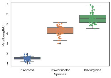
Now, let's plot the Box Plot and Strip Plot with Species on X_Axis and PetalLength on Y_Axis.
sns.boxplot(x="Species", y="PetalLengthCm", data=iris)
Output:
<AxesSubplot:xlabel='Species', ylabel='PetalLengthCm'>
ax = sns.boxplot(x="Species", y="PetalLengthCm", data=iris)
ax = sns.stripplot(x="Species", y="PetalLengthCm", data=iris, jitter=True, edgecolor="gray")
Output:
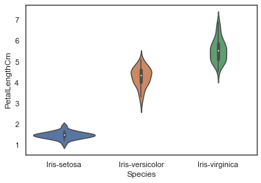
Now, Let's plot the same data with Violin Plot.
sns.violinplot(x="Species", y="PetalLengthCm", data=iris, size=6)
Output:
<AxesSubplot:xlabel='Species', ylabel='PetalLengthCm'>
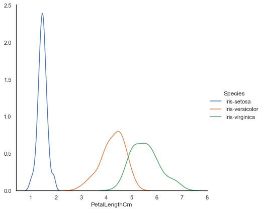
sns.FacetGrid(iris, hue="Species", size=6) \
   .map(sns.kdeplot, "PetalLengthCm") \
   .add_legend()
Output:
<seaborn.axisgrid.FacetGrid at 0x11c23130>
Now Pair Plot the data set.
sns.pairplot(iris.drop("Id", axis=1), hue="Species", size=3)
Output:
<seaborn.axisgrid.PairGrid at 0x11c17a90>
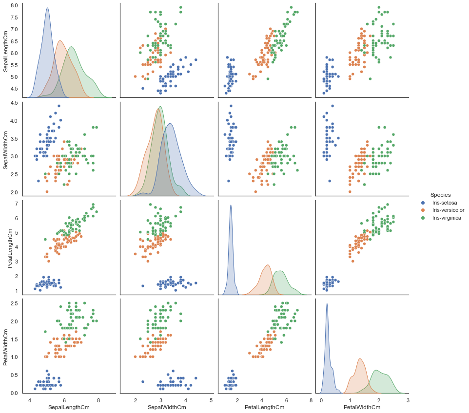
sns.pairplot(iris.drop("Id", axis=1), hue="Species", size=3, diag_kind="kde")
Output:
<seaborn.axisgrid.PairGrid at 0x124a8550>

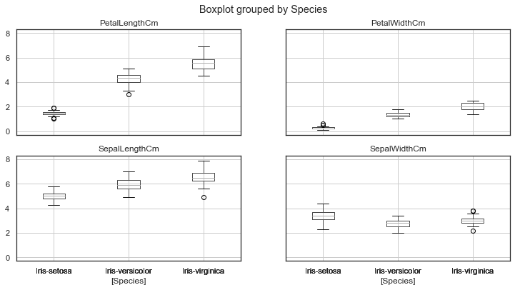
iris.drop("Id", axis=1).boxplot(by="Species", figsize=(12, 6))
array([[<AxesSubplot:title={'center':'PetalLengthCm'}, xlabel='[Species]'>,
        <AxesSubplot:title={'center':'PetalWidthCm'}, xlabel='[Species]'>],
       [<AxesSubplot:title={'center':'SepalLengthCm'}, xlabel='[Species]'>,
        <AxesSubplot:title={'center':'SepalWidthCm'}, xlabel='[Species]'>]],
      dtype=object)
Output:
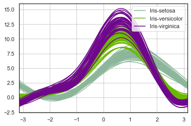
from pandas.plotting import andrews_curves
andrews_curves(iris.drop("Id", axis=1), "Species")
Output:
<AxesSubplot:>
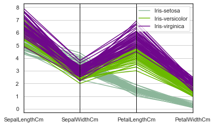
from pandas.plotting import parallel_coordinates
parallel_coordinates(iris.drop("Id", axis=1), "Species")
Output:
<AxesSubplot:>
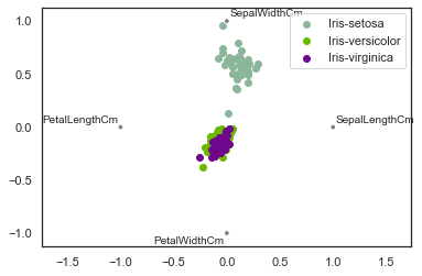
from pandas.plotting import radviz
radviz(iris.drop("Id", axis=1), "Species")
Output:
<AxesSubplot:>
Thank You!


